
Spot Instances are slowly but surely gaining traction with the enterprise AWS users. Who would want to lose out on a potential savings of up to 90% over On-Demand costs? Not me. Neither should you.
In this post, I will explain the basics of Spot Fleet and how it eases the use of native Spot Instances. I will also delve a bit into the missing pieces of Spot Fleet.
Spot Instances
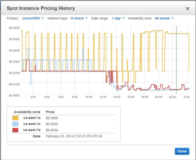
As you are already aware, Spot Instances are spare computing capacity available at deeply discounted prices. AWS allows users to bid on unused EC2 capacity in a region at any given point and run those instances for as long as their bid exceeds the current Spot Price. The Spot Price changes periodically based on supply and demand, and all users bids that meet or exceed it gain access to the available Spot Instances.
Provisioning Spot Instances in the hundreds and thousands is easy; AWS gives a single API call to do that. However, terminating them is a bit of pain! You need to hit terminate API call individually identified by their Spot Request Id ( which is in the format sir-xxxxxxxx).
Spot Fleet
In mid-2015, AWS announced Spot Fleet to make the EC2 Spot Instance model even more useful. With the addition of a new API, Spot Fleet allowed one to launch and manage an entire fleet of Spot Instances with just one request.
AWS defines Spot Fleet as, “…a collection, or fleet, of Spot instances. The Spot fleet attempts to launch the number of Spot instances that are required to meet the target capacity that you specified in the Spot fleet request. The Spot fleet also attempts to maintain its target capacity fleet if your Spot instances are interrupted due to a change in Spot prices or available capacity.”
Trend
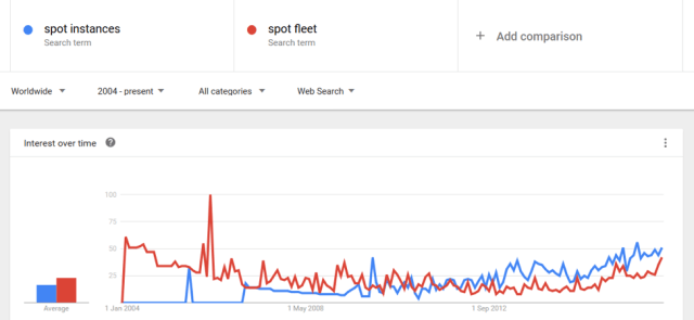
Google Trends shows that the awareness of both Spot Instances and Spot Fleet go hand-in-hand. What are the missing pieces then? Read on. But first, let’s understand the workings of Spot Fleet and how it is a boon for using Spot Instances.
Behind the scenes
Each Spot Fleet request must contain the following values:
- Target Capacity
- The number of Spot Instances you would want to launch
- Launch Specification
- The types of Spot Instances that you would want to launch and how you want them to be configured (AMI, VPC, subnets, Availability Zones, user data, security groups, and so on)
- Allocation Strategy
- It determines how it fulfills your Spot Fleet request from the possible Spot Instance pools represented by its Launch Specifications
- Lowest price
- Diversified
- It determines how it fulfills your Spot Fleet request from the possible Spot Instance pools represented by its Launch Specifications
- Maximum Bid Price
- The maximum bid price that you are willing to pay for all selected instance types.
- USD is the only accepted currency
A single Spot Fleet request gives us the power to launch thousands of Spot Instances and also be able to manage them. If a certain Spot Instance is terminated, then it is the responsibility of Spot Fleet to automatically launch a new one to maintain the Target Capacity.
Let’s go a little deep into the Allocation Strategy. It provides us with two options: lowestPrice and diversified. If your use-case is that of load testing for a couple of hours, then the probability of Spot Instances taken away from you is low, even with all instances in a single Spot Instance pool. lowestPrice strategy is a good choice for you as it provides the lowest cost.
Consider a use-case of an API endpoint running continuously without any tolerance for downtime with a target capacity of 50. If the allocation strategy is diversified spread across 5 Spot Instance pools, then it means that 10 Spot Instances will be provisioned in each pool. If the Spot price for one pool increases above your bid price for this pool, only 10% of your Spot Fleet is affected. Using diversified strategy gives you high availability as well as makes Spot Fleet less sensitive to increases in Spot Prices.
Spot Fleet also provides a feature called Instance Weighting, which will not be discussed in this blog post.
To better understand how Spot Instances are provisioned using the specified allocation strategy, I have reproduced a snippet from AWS docs:
- With the lowestPrice strategy (which is the default strategy), the Spot instances come from the pool with the lowest Spot price per unit at the time of fulfillment. To provide 20 units of capacity, the Spot fleet launches either 20 2xlarge instances (20 divided by 1), 10 r3.4xlarge instances (20 divided by 2), or 5 r3.8xlarge instances (20 divided by 4).
- With the diversified strategy, the Spot instances would come from all three pools. The Spot fleet would launch 6 2xlarge instances (which provide 6 units), 3 r3.4xlarge instances (which provide 6 units), and 2 r3.8xlarge instances (which provide 8 units), for a total of 20 units.
As you can clearly see, Spot Fleet makes the management of Spot Instances super simple. It also gives advanced features to better address issues related to high availability and specified target capacity. It really is a boon for all those using Spot Instances!
The Missing Pieces
Spot Fleet is great, no doubt. You have read all about the good features that it provides. You finally decide to take the plunge and use it in your application. Sooner than later, you realize that there are some gaps or situations where it can be difficult to use spot fleet.
- Native support to attach Spot Fleet instances to an ELB
- This is more of a convenience factor.
- As of now, the only way is via user-data scripts which the user has to write.
- Spot Fleet should take as input the ELB information to attach the provisioned Spot Instances.
- Spot Fleet should also take as input the record set information so as to give vanity URLs via Route53, provided the Hosted Zone and zone apex information is already configured.
- Fallback to on-demand instances
- This is not a Spot Fleet feature per se.
- It is more of a comfort factor.
- If Spot Fleet request can take as input the percentage distribution between on-demand and Spot Instances, then the application uptime is always guaranteed. So is the customers’ peace of mind.
I completely understand if you say, “Spot management is none of my business.” But, quite frankly, it is ours! Register now for a free 14-day trial of Batchly.
Remember: A penny saved is a penny earned!
X-Post from cmpute.io blog


